What's new in SQL Server 2022
Note: It seems since this post was written, some functions have been added, or some syntax has changed. So until I have time to update this post with the latest information, keep that in mind.
I’ve been excited to play with the new features and language enhancements in SQL Server 2022 so I’ve been keeping an eye on the Microsoft Docker repository for the 2022 image. Well they finally added it! I immediately pulled the image and started playing with it.
I want to focus on the language enhancements as those are the easiest to demonstrate, and I feel that’s what you’ll be able to take advantage of the quickest after upgrading.
Here’s the official post from Microsoft.
Table of contents:
- Docker Tag
- GENERATE_SERIES()
- GREATEST() and LEAST()
- STRING_SPLIT()
- DATE_BUCKET()
- FIRST_VALUE() and LAST_VALUE()
- WINDOW clause
- JSON functions
- Wrapping up
Docker Tag
I won’t go into the details of how to set up or use Docker, but you should definitely set aside some time to learn it. You can copy paste the command supplied by Microsoft on their Docker Hub page for SQL Server, but this is the one I prefer to use:
docker run -it `
    --name sqlserver `
    -e ACCEPT_EULA='Y' `
    -e MSSQL_SA_PASSWORD='yourStrong(!)Password' `
    -e MSSQL_AGENT_ENABLED='True' `
    -p 1433:1433 `
    mcr.microsoft.com/mssql/server:2022-latest;
This sets it up to always use the same name of “sqlserver” for the container, this keeps you from creating multiple SQL server containers. It keeps it in interactive mode so you can watch for system errors, and it starts it up with SQL Agent running. Also, this will automatically download and run the SQL Server image if you don’t already have it.
You won’t need to worry about loading up any specific databases for this blog post, but if that’s something you’d like to learn how to do, I’ve blogged about it here.
GENERATE_SERIES()
I want to cover this function first so we can use it to help us with building sample data for the rest of this post.
Generating a series of incrementing (or decrementing) values is extremely useful. If you’ve never used a “tally table” or a “numbers table” plenty of other SQL bloggers have covered it and I highly recommend looking up their posts.
A few uses for tally tables:
-
Can often be the solution that avoids reverting to what Jeff Moden likes to call “RBAR”…Row-By-Agonizing-Row. Tally tables can help you perform iterative / incremental tasks without having to build any looping mechanisms. In fact, one of the fastest solutions for splitting strings (prior to
STRING_SPLIT()) is using a tally table. Up until recently (we’ll cover that later), that tally table string split function was still one of the best methods even despiteSTRING_SPLIT()being available. -
Can help you with reporting, such as building a list of dates so that you don’t have gaps in your aggregated report that is grouped by day or month. If you group sales by month, but a particular month had no sales you can use the tally table to fill the gaps with “0” sales.
-
They’re great for helping you generate sample data as you’ll see throughout this post.
Prior to this new function, the best way I’ve seen to generate a tally table is using the CTE method, like so:
WITH c1 AS (SELECT x.x FROM (VALUES(1),(1),(1),(1),(1),(1),(1),(1),(1),(1)) x(x))  -- 10
    , c2(x) AS (SELECT 1 FROM c1 x CROSS JOIN c1 y)                                -- 10 * 10
    , c3(x) AS (SELECT 1 FROM c2 x CROSS JOIN c2 y CROSS JOIN c2 z)                -- 100 * 100 * 100
    , c4(rn) AS (SELECT 0 UNION SELECT ROW_NUMBER() OVER (ORDER BY (SELECT 1)) FROM c3)  -- Add zero record, and row numbers
SELECT TOP(1000) x.rn
FROM c4 x
ORDER BY x.rn;
This will generate rows with values from 0 to 1,000,000. In this sample, it is using a TOP(1000) and an ORDER BY to only return the first 1,000 rows (0 - 999). It can be easily modified to generate more or less rows or ranges of rows and it’s extremely fast.
Another method I personally figured out while trying to work on a code golf problem was using XML:
DECLARE @x xml = REPLICATE(CONVERT(varchar(MAX),'<n/>'), 999); --Table size
WITH c(rn) AS (
    SELECT 0
    UNION ALL
    SELECT ROW_NUMBER() OVER (ORDER BY (SELECT 1))
    FROM @x.nodes('n') x(n)
)
SELECT c.rn
FROM c;
This method is more for fun, and I typically wouldn’t use this in a production environment. I’m sure it’s plenty stable, I just prefer the CTE method more. This method also returns 1000 records (0 - 999).
Now, in comes the GENERATE_SERIES() function. You specify where it starts, where it ends and what to increment by (optional). Though, this is certainly not a direct drop in replacement for the options above and I’ll show you why.
SELECT [value]
FROM GENERATE_SERIES(START = 0, STOP = 999, STEP = 1);
This is pretty awesome, and it definitely beats typing all that other junk from the other options and it’s a lot more straight forward and intuitive to read.
I think it’s great that you can customize it to increment, decrement, change the range and even change the datatype by supplying decimal values. You can also set the “STEP” size (i.e. only return every N values). I could see this coming in handy for generating date tables. For example, generate a list of dates going back every 30 days or every 14 days.
-- List of dates going back every 30 days for 180 days
SELECT DateValue = CONVERT(date, DATEADD(DAY, [value], '2022-06-01'))
FROM GENERATE_SERIES(START = -30, STOP = -180, STEP = -30);

/* Result:
| DateValue  |
|------------|
| 2022-05-02 |
| 2022-04-02 |
| 2022-03-03 |
| 2022-02-01 |
| 2022-01-02 |
| 2021-12-03 |
*/
You could certainly do this with the CTE method, it just wouldn’t be as obvious as this.
However, I quickly discovered one major caveat…performance. This GENERATE_SERIES() function is an absolute pig 🐷. I don’t know why it’s so slow, maybe they’re still working out the kinks, or maybe it will improve in a future update.
Here’s how it stacks up on my local machine in docker.
Generating 1,000,001 rows from 0 to 1,000,000:
| Method | CPU Time (ms) | Elapsed Time (ms) |
|---|---|---|
| CTE | 1,361 | 500 |
| XML | 775 | 784 |
GENERATE_SERIES() |
47,801 | 44,371 |
Unless there’s something wrong with my docker image…this doesn’t seem ready for prime time. I could see this being used in utility scripts, sample scripts (like this blog post), reporting procs, etc. Where you only need to generate a small set of records, but if you need to generate a large set of records often, it seems you’re best sticking with the CTE method for now.
I could possibly see this being useful when used inline where you need to generate a different number of records for each row (e.g. in an APPLY operator). However, even then, seeing how slow this is, you might be better off building your own TVF using the CTE method 🤷♂️. So while it may be shorter and much easier to use, I’m not sure if the performance trade-off is worth it. Hopefully it’s just my machine?
Now that we’ve got this one out of the way, we can use it to help us with generating sample data for the rest of this post.
GREATEST() and LEAST()
Microsoft Documentation:
These are not exactly new. They have made their way around the blogging community for a while after they were discovered as undocumented functions in Azure SQL Database, but they’re still worth demonstrating since they are part of the official 2022 release changes.
I’m sure all of you know how to use MIN() and MAX(). These are aggregate functions that run against a grouping, or a window. Their usage is fairly straight forward. If you want to find the highest or lowest value for a single column in a GROUP BY or a window function, you would use one of those.
But what if you want to get the highest or lowest value from multiple columns within a row? For example, maybe you have LastModifiedDate, LastAccessDate and LastErrorDate columns and you want the most recent date in order to determine the last interaction with that item?
Previously, you’d need to use a case statement or a table value constructor.
It would look something like this:
-- Generate sample data

DROP TABLE IF EXISTS #event;
CREATE TABLE #event (
    ID                  int     NOT NULL IDENTITY(1,1),
    LastModifiedDate    datetime    NULL,
    LastAccessDate      datetime    NULL,
    LastErrorDate       datetime    NULL,
);

INSERT INTO #event (LastModifiedDate, LastAccessDate, LastErrorDate)
SELECT DATEADD(SECOND, -(RAND(CHECKSUM(NEWID())) * 200000000), GETDATE())
    ,  DATEADD(SECOND, -(RAND(CHECKSUM(NEWID())) * 200000000), GETDATE())
    ,  DATEADD(SECOND, -(RAND(CHECKSUM(NEWID())) * 200000000), GETDATE())
FROM GENERATE_SERIES(START = 1, STOP = 5); -- See...nifty, right?
-- Old method using table value constructor
SELECT LastModifiedDate, LastAccessDate, LastErrorDate
    , y.[Greatest], y.[Least]
FROM #event
    CROSS APPLY (
        SELECT [Least] = MIN(x.val), [Greatest] = MAX(x.val)
        FROM (VALUES (LastModifiedDate), (LastAccessDate), (LastErrorDate)) x(val)
    ) y;

-- New method using LEAST/GREATEST functions
SELECT LastModifiedDate, LastAccessDate, LastErrorDate
    , [Greatest] = GREATEST(LastModifiedDate, LastAccessDate, LastErrorDate)
    , [Least]    = LEAST(LastModifiedDate, LastAccessDate, LastErrorDate)
FROM #event;
Result:
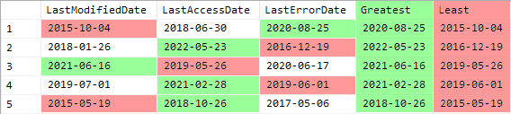
Of course this also comes with a caveat. These new functions are great if all you want to do is find the highest or lowest value…but if you want to use any other aggregate function, like AVG() or SUM()…unfortunately you’d still need to use the old method.
STRING_SPLIT()
This is also not a new function, however, after (I’m sure) many requests…it has been enhanced. Most people probably don’t know, or maybe just haven’t bothered to care, but up until now, you should never rely on the order that STRING_SPLIT() returns its results. They are not considered to be returned in any particular order, and that is still the case.
However, they have now added an additional “ordinal” column that you can turn on using an optional setting.
Before, you would often seen people use STRING_SPLIT() like this:
SELECT [value], ordinal
FROM (
    SELECT [value]
        , ordinal = ROW_NUMBER() OVER (ORDER BY (SELECT NULL))
    FROM STRING_SPLIT('one fish,two fish,red fish,blue fish', ',')
) x;

/* Result:
| value     | ordinal |
|-----------|---------|
| one fish  | 1       |
| two fish  | 2       |
| red fish  | 3       |
| blue fish | 4       |
*/
And while you more than likely will get the right numbers associated with the correct position of the item…you really shouldn’t do this because it’s undocumented behavior. At any time, Microsoft could change how this function works internally, and now all of a sudden that production code you wrote relying on its order is messing up.
But now you can enable an “ordinal” column to be included in the output. The value of the column indicates the order in which the item occurs in the string.
SELECT [value], ordinal
FROM STRING_SPLIT('one fish,two fish,red fish,blue fish', ',', 1);

/* Result:
| value     | ordinal |
|-----------|---------|
| one fish  | 1       |
| two fish  | 2       |
| red fish  | 3       |
| blue fish | 4       |
*/
DATE_BUCKET()
Now this is a cool new function that I’m looking forward to testing out. It’s able to give you the beginning of a date range based on the interval you provide it. For example “what’s the first day of the month for this date”.
Simple usage:
DECLARE @date datetime = GETDATE();
SELECT Interval, [Value]
FROM (VALUES
      ('Source' , @date)
    , ('SECOND' , DATE_BUCKET(SECOND , 1, @date))
    , ('MINUTE' , DATE_BUCKET(MINUTE , 1, @date))
    , ('HOUR'   , DATE_BUCKET(HOUR   , 1, @date))
    , ('DAY'    , DATE_BUCKET(DAY    , 1, @date))
    , ('WEEK'   , DATE_BUCKET(WEEK   , 1, @date))
    , ('MONTH'  , DATE_BUCKET(MONTH  , 1, @date))
    , ('QUARTER', DATE_BUCKET(QUARTER, 1, @date))
    , ('YEAR'   , DATE_BUCKET(YEAR   , 1, @date))
) x(Interval, [Value]);

/* Result:
| Interval | Value                   |
|----------|-------------------------|
| Source   | 2022-06-02 13:30:48.353 |
| SECOND   | 2022-06-02 13:30:48.000 |
| MINUTE   | 2022-06-02 13:30:00.000 |
| HOUR     | 2022-06-02 13:00:00.000 |
| DAY      | 2022-06-02 00:00:00.000 |
| WEEK     | 2022-05-30 00:00:00.000 |
| MONTH    | 2022-06-01 00:00:00.000 |
| QUARTER  | 2022-04-01 00:00:00.000 |
| YEAR     | 2022-01-01 00:00:00.000 |
*/
See how each interval is being rounded down to the nearest occurrence? This is super useful for things like grouping data by month. For example, “group sales by month using purchase date”. Prior to this you’d have to use methods like the following:
SELECT DATEPART(MONTH, PurchaseDate), DATEPART(YEAR, PurchaseDate)
FROM dbo.Sale
GROUP BY DATEPART(MONTH, PurchaseDate), DATEPART(YEAR, PurchaseDate);

--OR

SELECT MONTH(PurchaseDate), YEAR(PurchaseDate)
FROM dbo.Sale
GROUP BY MONTH(PurchaseDate), YEAR(PurchaseDate);
Those work, but they’re ugly, because now you have a column for month and a column for year. So then you might use something like:
SELECT DATEFROMPARTS(YEAR(PurchaseDate), MONTH(PurchaseDate), 1)
FROM dbo.Sale
GROUP BY DATEFROMPARTS(YEAR(PurchaseDate), MONTH(PurchaseDate), 1);

--OR

SELECT DATEADD(MONTH, DATEDIFF(MONTH, 0, GETDATE()), 0)
FROM dbo.Sale
GROUP BY DATEADD(MONTH, DATEDIFF(MONTH, 0, GETDATE()), 0);
These methods work too…but they’re both a bit ugly, especially that second method. But that second method comes in handy when you need to use other intervals, like WEEK or QUARTER because then the DATEFROMPARTS() method doesn’t work.
So rather than using all those old methods, now you can use:
SELECT DATE_BUCKET(MONTH, 1, PurchaseDate)
FROM dbo.Sale
GROUP BY DATE_BUCKET(MONTH, 1, PurchaseDate);
Easy as that. Easier to read, easier to know what it’s doing.
It also allows you to specify a “bucket width”. To put it in plain terms, it allows you to round down to the nearest increment of time. For example, you could use it to round down to the nearest interval of 5 minutes. So 06:33:34 rounds down to 06:30:00. This is great for reporting. You can break data up into chunks, for example, maybe you want to break the day up into 8 hour shifts.
DROP TABLE IF EXISTS #log;
CREATE TABLE #log (
    InsertDate datetime NULL,
);

-- Generate 1000 events with random times spread out across a single day
INSERT INTO #log (InsertDate)
SELECT DATEADD(SECOND, -(RAND(CHECKSUM(NEWID())) * 86400), '2022-06-02')
FROM GENERATE_SERIES(START = 1, STOP = 1000); -- I told you this would be useful

SELECT TOP(5) InsertDate FROM #log;
/*
| InsertDate              |
|-------------------------|
| 2022-06-01 19:22:54.000 |
| 2022-06-01 08:01:13.000 |
| 2022-06-01 09:35:48.000 |
| 2022-06-01 22:28:38.000 |
| 2022-06-01 05:26:08.000 |
*/
In this example, I’ve generate 1,000 random events to simulate a log table. Prior to using DATE_BUCKET() how would you have broken this up into 8 hour chunks? Here’s how I would have done it:
SELECT DATEADD(HOUR, (DATEDIFF(HOUR, 0, InsertDate) / 8) * 8, 0)
    , Total = COUNT(*)
FROM #log
GROUP BY DATEADD(HOUR, (DATEDIFF(HOUR, 0, InsertDate) / 8) * 8, 0);
All this is doing is getting the number of hours since 1900-01-01 (0), then dividing by 8. Since I’m dividing an int by an int, it automatically floors the result. So 10 / 8 = 1, 15 / 8 = 1, 16 / 8 = 2, otherwise you would need to explicitly use FLOOR(). Then it is re-adding those hours back to 0 to get the datetime rounded to the nearest increment of 8 hours. Fortunately, increments of 2, 3, 4, 6, 8 and 12 all work nicely with this method.
However, DATE_BUCKET() makes this a lot easier:
SELECT Bucket = DATE_BUCKET(HOUR, 8, InsertDate)
    , Total = COUNT(*)
FROM #log
GROUP BY DATE_BUCKET(HOUR, 8, InsertDate);

/* Result:
| Bucket                  | Total |
|-------------------------|-------|
| 2022-06-01 00:00:00.000 | 378   |
| 2022-06-01 08:00:00.000 | 303   |
| 2022-06-01 16:00:00.000 | 319   |
*/
FIRST_VALUE() and LAST_VALUE()
Microsoft Documentation:
Similar to SPLIT_STRING(), neither of these are new, but they have been greatly enhanced. After years of waiting, we finally have the ability to control how NULL values are handled with the use of IGNORE NULLS and RESPECT NULLS.
In SQL Server, NULL values are always sorted to the “lowest” end. So if you sort ascending, NULL values will be at the top. Unfortunately, we don’t have a choice over that matter. In other RDBMSs such as Postgres, you can control this behavior (e.g. ORDER BY MyValue ASC NULLS LAST).
I’ve personally never run into this as a major problem, there’s always ways around it, such as ORDER BY IIF(MyValue IS NULL, 0, 1), MyValue, which will sort NULL values to the bottom first, then sort by MyValue.
In a similar way, you can run into issues with this when using FIRST_VALUE() or LAST_VALUE() and the data contains NULL values. It’s not exactly the same issue, but it goes along the same lines as having control over how NULL values are treated.
I was going to build a example for this, but then I ran across this article from Microsoft, which uses the exact example I was going to build, and it perfectly explains and demonstrates how you can use this new feature to fill in missing data using IGNORE NULLS:
https://docs.microsoft.com/en-us/azure/azure-sql-edge/imputing-missing-values
WINDOW clause
I’m honestly very surprised that this was included, but I’m glad it was. If you’re familiar with using window functions, then you are going to love this.
Let’s use a very simple example. I’m going to use GENERATE_SERIES() to get a list of values 1 - 10. Now I want to perform some window operations on those values, partitioning them by odd vs even. So for both odd and even numbers, I want to see a row number, a running total (sum), a running count, and a running average.
SELECT [value]
    , RowNum = ROW_NUMBER() OVER (PARTITION BY [value] % 2 ORDER BY [value])
    , RunSum = SUM([value]) OVER (PARTITION BY [value] % 2 ORDER BY [value])
    , RunCnt = COUNT(*)     OVER (PARTITION BY [value] % 2 ORDER BY [value])
    , RunAvg = AVG([value]) OVER (PARTITION BY [value] % 2 ORDER BY [value])
FROM GENERATE_SERIES(START = 1, STOP = 10)
ORDER BY [value];

/* Result:
| value | RowNum | RunSum | RunCnt | RunAvg |
|-------|--------|--------|--------|--------|
| 1     | 1      | 1      | 1      | 1      |
| 2     | 1      | 2      | 1      | 2      |
| 3     | 2      | 4      | 2      | 2      |
| 4     | 2      | 6      | 2      | 3      |
| 5     | 3      | 9      | 3      | 3      |
| 6     | 3      | 12     | 3      | 4      |
| 7     | 4      | 16     | 4      | 4      |
| 8     | 4      | 20     | 4      | 5      |
| 9     | 5      | 25     | 5      | 5      |
| 10    | 5      | 30     | 5      | 6      |
*/
The problem here is we’re repeating a lot of code…OVER (PARTITION BY [value] % 2 ORDER BY [value]) is repeated four times. That’s a bit wasteful, and open to error. All it takes is for that window to change and a developer accidentally forgets to update one of them.
That’s where the new WINDOW clause comes in. Instead, you can define your window with a name/alias and then reuse it. So it is only defined once.
SELECT [value]
    , RowNum = ROW_NUMBER() OVER win
    , RunSum = SUM([value]) OVER win
    , RunCnt = COUNT(*)     OVER win
    , RunAvg = AVG([value]) OVER win
FROM GENERATE_SERIES(START = 1, STOP = 10)
WINDOW win AS (PARTITION BY [value] % 2 ORDER BY [value])
ORDER BY [value];
I love how simple this is. Now our window is defined only once. Any future changes only need to alter a single line. I’m looking forward to using this one.
JSON functions
I saved this section for last on purpose because I have almost no experience working with JSON so I likely won’t have great real-world examples, but I can at least walk through the usage of these functions.
Microsoft has great examples in their documentation already, so this walk-through is more for me than you because it’s forcing me to learn how to use these functions.
Microsoft Documentation:
ISJSON()
The ISJSON() function is not new (thank you to the reddit user that pointed this out to me), but it was enhanced. There is now a json_type_constraint parameter.
Without the new parameter, this one is about as simple as it gets…It checks whether the value you pass is valid JSON or not.
SELECT ISJSON('{ "name":"Chad" }'); -- Returns 1 because it is valid JSON
SELECT ISJSON('{ name:"Chad" }');   -- Returns 0 because it is invalid JSON
However, the new parameter allows you to do a little more than just check whether the blob you pass to it is valid or not. Now you can check if its type is valid as well. Maybe you’re generating JSON and you want to test the individual parts rather than testing the entire blob at the end of your task.
Here are some test cases:
SELECT *
FROM (VALUES  ('string','"testing"'), ('empty string','""'), ('bad string','asdf')
            , ('scalar','1234')
            , ('boolean','true'), ('bad boolean', 'TRUE')
            , ('array','[1,2,{"foo":"bar"}]'), ('empty array', '[]')
            , ('object','{"name":"chad"}'), ('empty object','{}')
            , ('null literal','null')
            , ('blank value', '')
            , ('NULL value', NULL)
) x([type], [value])
    CROSS APPLY (
        -- Case statements to make visualization of results easier
        SELECT [VALUE]  = CASE ISJSON(x.[value], VALUE)  WHEN 1 THEN 'True' WHEN 0 THEN '' ELSE NULL END
            ,  [SCALAR] = CASE ISJSON(x.[value], SCALAR) WHEN 1 THEN 'True' WHEN 0 THEN '' ELSE NULL END
            ,  [ARRAY]  = CASE ISJSON(x.[value], ARRAY)  WHEN 1 THEN 'True' WHEN 0 THEN '' ELSE NULL END
            ,  [OBJECT] = CASE ISJSON(x.[value], OBJECT) WHEN 1 THEN 'True' WHEN 0 THEN '' ELSE NULL END
    ) y

/* Result:
| type         | value               | VALUE | SCALAR | ARRAY | OBJECT |
|--------------|---------------------|-------|--------|-------|--------|
| string       | "testing"           | True  | True   |       |        |
| empty string | ""                  | True  | True   |       |        |
| bad string   | asdf                |       |        |       |        |
| scalar       | 1234                | True  | True   |       |        |
| boolean      | true                | True  |        |       |        |
| bad boolean  | TRUE                |       |        |       |        |
| array        | [1,2,{"foo":"bar"}] | True  |        | True  |        |
| empty array  | []                  | True  |        | True  |        |
| object       | {"name":"chad"}     | True  |        |       | True   |
| empty object | {}                  | True  |        |       | True   |
| null literal | null                | True  |        |       |        |
| blank value  |                     |       |        |       |        |
| NULL value   | NULL                | NULL  | NULL   | NULL  | NULL   |
*/
Based on these results you can see that VALUE is a generic check, determining whether the value is valid regardless of type. Whereas SCALAR, ARRAY and OBJECT are more granular and check for specific types.
JSON_PATH_EXISTS()
Checks to see whether the path you specify exists in the provided JSON blob.
DECLARE @jsonblob nvarchar(MAX) = N'
{
    "name":"Chad Baldwin",
    "addresses":[
        {"type":"billing", "street":"123 Main Street", "city":"New York", "state":"NY", "zip":"01234"},
        {"type":"shipping", "street":"2073 Beech Street", "city":"Pleasanton", "state":"CA", "zip":"94566"}
    ]
}';

SELECT ISJSON(@jsonblob); -- returns 1 because it is valid JSON
SELECT JSON_PATH_EXISTS(@jsonblob, '$.addresses[0].zip'); -- returns 1 because the path exists
Explanation of $.addresses[0].zip:
$- represents the root of the blobaddresses[0]- returns the first object within theaddressesarray.zip- looks for a property namedzipwithin that object
JSON_OBJECT()
This is an interesting one, the syntax is a bit odd, but you’re basically passing the function key:value pairs, which it then uses to build a simple JSON string.
SELECT item = x.y, jsonstring = JSON_OBJECT('item':x.y)
FROM (VALUES ('one fish'),('two fish'),('red fish'),('blue fish')) x(y);

/* Result:
| item      | jsonstring           |
|-----------|----------------------|
| one fish  | {"item":"one fish"}  |
| two fish  | {"item":"two fish"}  |
| red fish  | {"item":"red fish"}  |
| blue fish | {"item":"blue fish"} |
*/
So it allows you to generate a JSON object for a set of values/columns on a per row basis.
JSON_ARRAY()
This is similar as JSON_OBJECT() in regard to generating JSON from data, except instead of creating an object with various properties, it’s creating an array of values or objects.
SELECT JSON_ARRAY('one fish','two fish','red fish','blue fish');

/* Result:
["one fish","two fish","red fish","blue fish"]
*/
From there you can combine JSON_OBJECT and JSON_ARRAY to generate nested JSON blobs from your data.
Wrapping up
This ended up being much longer than I had originally anticipated, but I’m glad I went through it as it helped me gain a much better understanding of all these changes, new functions, enhancements, and how to use them in real world situations.
Thanks for reading!